DEPARTMENT OF PSYCHOLOGY, NORTHWESTERN UNIVERSITY
RICHARD E. ZINBARG
DEPARTMENT OF PSYCHOLOGY, THE FAMILY INSTITUTE AT NORTHWESTERN
UNIVERSITY, NORTHWESTERN UNIVERSITY
Keywords: reliability, internal consistency, homogeneity, test theory, coefficient alpha, coefficient omega, coefficient beta.
Rephrasing Spearman (1904, 1910) in more current terminology (Lord & Novick, 1968; McDonald, 1999), reliability is the correlation between two parallel tests where tests are said to be parallel if for every subject, the true scores on each test are the expected scores across an infinite number of tests, and thus the same, and the error variances across subjects for each test are the same. Unfortunately, “all measurement is befuddled by error” (McNemar, 1946, p. 294).
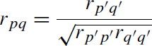
Error may be defined as observed score−true score, and hence to be uncorrelated with true score and uncorrelated across tests. Thus, reliability is the fraction of test variance that is true score variance. However, such a definition requires finding a parallel test. For just knowing the correlation between two tests, without knowing the true scores or their variance (and if we did, we would not bother with reliability), we are faced with three knowns (two variances and one covariance), but ten unknowns (four variances and six covariances).
In this case of two tests, by defining them to be parallel with uncorrelated errors, the number of unknowns drops to three and reliability of each test may be found.With three tests, the number of assumptions may be reduced, and if the tests are tau (τ ) equivalent (each test has the same true score covariance), reliability for each of the three tests may be found.With four tests, to find the reliability of each test, we need only assume that the tests all measure the same construct (to be “congeneric”), although possibly with different true score and error score variances (Lord & Novick, 1968).
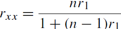
Subsequent efforts were based on the domain sampling model in which tests are seen as being made up of items randomly sampled from a domain of items (Lord, 1955, made the distinction between “Type 1” sampling of people, “Type 2” sampling of items, and “Type 12” sampling of persons and items). The desire for an easy to use “magic bullet” based upon the domain sampling model has led to a number of solutions (e.g., the six considered by Guttman, 1945), of which one, coefficient alpha (Cronbach, 1951) is easy to compute and easy to understand. The appeal of α was perhaps that it was the average of all such random splits (Cronbach, 1951).
Even though the pages of Psychometrika have been filled over the years with critiques and cautions about coefficient α and have seen elegant solutions for more appropriate estimates, few of these suggested coefficients are used. This is partly because they are not easily available in programs for the end user nor described in a language that is accessible to many psychologists. In a statement reminiscent of Spearman’s observation that “Psychologists, with scarely an exception, never seem to have become acquainted with the brilliant work being carried on since 1886 by the Galton–Pearson school” (Spearman, 1904, p. 96), Sijtsma (2008) points out that psychometrics and psychology have drifted apart as psychometrics has become more statistical and psychologists have remained psychologists.Without clear discussions of the alternatives and easily available programs to find the alternative estimates of reliability, most psychologists will continue to use α. With the advent of open source programming environments for statistics such as R (R Development Core Team, 2008), that are easy to access and straightforward to use, it is possible that the other estimates of reliability will become more commonly used.
What coefficients should we use? Sijtsma (2008) reviews a hierarchy of lower bound estimates of reliability and in agreement with Jackson and Agunwamba (1977) and Woodhouse and Jackson (1977) suggests that the glb or “greatest lower bound” (Bentler & Woodward, 1980) is, in fact, the best estimate. We believe that this is an inappropriate suggestion for at least three reasons:
- Contrary to what the name implies, the glb is not the greatest lower bound estimate of reliability, but is somewhat less than another, easily calculated and understood estimate of reliability (ωtotal,ωt) of McDonald (1999). (We use the subscript on ωt to distinguish between the coefficient ω introduced by McDonald (1978), equation (9), and McDonald (1999), equation (6.20) that he also called ω and which we (Zinbarg, Revelle, & Yovel, 2005) previously relabeled ωhierarchical,ωh).
- Rather than just focusing on the greatest lower bounds as estimates of a reliability of a test, we should also be concerned with the percentage of the test that measures one construct. As has been discussed previously (Revelle, 1979; McDonald, 1999; Zinbarg et al., 2005), this may be estimated by finding ωh, the general factor saturation of the test (McDonald, 1999; Zinbarg et al., 2005), or the worst split half reliability of a test (coefficient beta, β, of Revelle, 1979).
- Although it is easy to estimate all of the Guttman (1945) lower bounds, as well as β, ωh, and ωt, the techniques for estimating the glb are not readily available for the end user.
1. The Ordering of Reliability Estimates
Although arguing that reliability was only meaningful in the case of test-retest, Guttman (1945) may be credited with introducing a series of lower bounds for reliability, each based upon the item characteristics of a single test. These six have formed the base for most of the subsequent estimates.
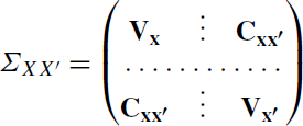
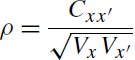
Vx = 1Vx1′ = 1Ct1′ + 1Ve1′ = Vt +Ve
and the structure of the two tests seen in (3) becomes